Graph Neural Networks with Learnable Structural and Positional Representations

该论文在拉普拉斯PE的基础上，新的可学习节点位置编码（PE），用于图嵌入。

（ICLR 2022）

为什么要使用位置编码

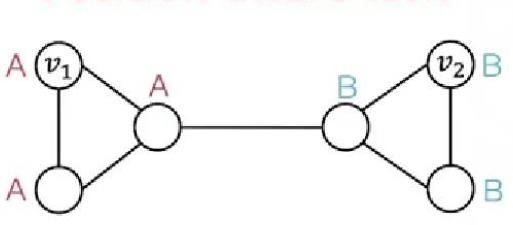
比如单靠信息传播，下图的结构并不能很好学习：

解决方案：

• 堆叠多层

由于过度压缩现象，它可能对远距离节点是不够的。

• 应用高阶

K 阶 WL-GNN 在扩展中比 MP-GNN 计算上更昂贵，即使对于中等规模的图也是如此。

• 考虑节点的位置编码（PE）（以及边的位置编码）

比如像graphormer（第一个Graph transfomrer），采用了三种位置编码：

（1）Centrality Encoding

即

node_feature = (
    node_feature
    + nn.Embedding()(in_degree)
    + nn.Embedding()(out_degree)
)

（2）Spatial Encoding

给定一个合理的距离度量 ϕ(v_i, v_j), 根据两个节点(v_i, v_j)之间的距离，为其分配相应的编码向量。距离度量 ϕ(⋅) 的选择多种多样，对于一般性的图数据可以选择无权或带权的最短路径，而对于特别的图数据则可以有针对性的选择距离度量，例如物流节点之间的最大流量，化学分子 3D 结构中原子之间的欧氏距离等等。

为了不失一般性，Graphormer 在实验中采取了无权的最短路径作为空间编码的距离度量。

（3）Edge Encoding

在计算两个节点之间的相关性时，作者对这两个节点最短路径上的连边特征进行加权求和作为注意力偏置，其中权重是可学习的。

---

另外简单的还有比如Laplacian Eigenvectors as PE，但由于拉普拉斯矩阵的特征向量 v 和其相反向量 −v 都描述了相同的结构信息（因为它们对应同一个特征值）。当我们将这些特征向量用作节点的位置编码时，就会出现不唯一性。它可能会将这些实际上表示相同结构信息的编码视为完全不同的输入，从而影响学习效率和泛化能力。

代码分析

官方代码：https://github.com/vijaydwivedi75/gnn-lspe

写得有些混乱，我们不如直接看dgl的源码：https://www.dgl.ai/dgl_docs/_modules/dgl/transforms/functional.html#random_walk_pe

def random_walk_pe(g, k, eweight_name=None):
    r"""Random Walk Positional Encoding, as introduced in
    `Graph Neural Networks with Learnable Structural and Positional Representations
    <https://arxiv.org/abs/2110.07875>`__

    This function computes the random walk positional encodings as landing probabilities
    from 1-step to k-step, starting from each node to itself.

    Parameters
    ----------
    g : DGLGraph
        The input graph. Must be homogeneous.
    k : int
        The number of random walk steps. The paper found the best value to be 16 and 20
        for two experiments.
    eweight_name : str, optional
        The name to retrieve the edge weights. Default: None, not using the edge weights.

    Returns
    -------
    Tensor
        The random walk positional encodings of shape :math:`(N, k)`, where :math:`N` is the
        number of nodes in the input graph.

    Example
    -------
    >>> import dgl
    >>> g = dgl.graph(([0,1,1], [1,1,0]))
    >>> dgl.random_walk_pe(g, 2)
    tensor([[0.0000, 0.5000],
            [0.5000, 0.7500]])
    """
    N = g.num_nodes()  # number of nodes
    M = g.num_edges()  # number of edges
    A = g.adj_external(scipy_fmt="csr")  # adjacency matrix
    if eweight_name is not None:
        # add edge weights if required
        W = sparse.csr_matrix(
            (g.edata[eweight_name].squeeze(), g.find_edges(list(range(M)))),
            shape=(N, N),
        )
        A = A.multiply(W)
    # 1-step transition probability
    if version.parse(scipy.__version__) < version.parse("1.11.0"):
        RW = np.array(A / (A.sum(1) + 1e-30))
    else:
        # Sparse matrix divided by a dense array returns a sparse matrix in
        # scipy since 1.11.0.
        RW = (A / (A.sum(1) + 1e-30)).toarray()

    # Iterate for k steps
    PE = [F.astype(F.tensor(np.array(RW.diagonal())), F.float32)]
    RW_power = RW
    for _ in range(k - 1):
        RW_power = RW_power @ RW
        PE.append(F.astype(F.tensor(np.array(RW_power.diagonal())), F.float32))
    PE = F.stack(PE, dim=-1)

    return PE

g = dgl.graph(([0,1,1], [1,1,0])) 边: 0->1, 1->1 (自环), 1->0
对于这个 g，邻接矩阵 A (假设 MockDGLGraph 行为类似):
[[0, 1],
 [1, 1]]

N = 2, M = 3 (在 DGL 示例中，尽管 MockDGLGraph 可能根据其初始化方式不同地计算唯一边)
对于 g = MockDGLGraph(([0,1,1], [1,1,0])):
A = [[0, 1],
     [1, 1]] (节点0连接到1；节点1连接到0和1(自环))

A.sum(1):
第0行和 (节点0): 0 + 1 = 1
第1行和 (节点1): 1 + 1 = 2
所以, A.sum(1) = [[1], [2]] (作为列向量用于广播)

RW = A / A.sum(1):
RW_row0 = [0/1, 1/1] = [0, 1]
RW_row1 = [1/2, 1/2] = [0.5, 0.5]
RW = [[0.0, 1.0],
      [0.5, 0.5]]

初始 PE (1步返回概率):
RW.diagonal() = [0.0, 0.5]
PE = [[0.0, 0.5]] (概念上，在堆叠之前)

k = 2, 所以循环运行 k-1 = 1 次。
迭代 1 (计算2步概率):
RW_power = RW @ RW
RW_power = [[0.0, 1.0],  @  [[0.0, 1.0],
            [0.5, 0.5]]     [0.5, 0.5]]

RW_power[0,0] = (0.0 * 0.0) + (1.0 * 0.5) = 0.5
RW_power[0,1] = (0.0 * 1.0) + (1.0 * 0.5) = 0.5
RW_power[1,0] = (0.5 * 0.0) + (0.5 * 0.5) = 0.25
RW_power[1,1] = (0.5 * 1.0) + (0.5 * 0.5) = 0.5 + 0.25 = 0.75

RW_power (RW^2) = [[0.5 , 0.5 ],
                   [0.25, 0.75]]

RW_power (RW^2) 的对角线: [0.5, 0.75]
PE 列表变为: [[0.0, 0.5], [0.5, 0.75]] (概念上)

F.stack(PE, dim=-1):
堆叠 [0.0, 0.5] 和 [0.5, 0.75]
最终的 PE 张量:
[[0.0, 0.5 ],  <- 节点0: P(1步返回), P(2步返回)
 [0.5, 0.75]]  <- 节点1: P(1步返回), P(2步返回)

这与示例输出匹配:
tensor([[0.0000, 0.5000],
        [0.5000, 0.7500]])