Quasi-SVM

SVM是一个强有力的机器学习算法，很多算法（比如RCNN）的分类器也使用SVM作为分类器，帮助我获得了博弈杯准确率排行榜的第二名（我使用的是VGG+Quasi-SVM。

但困难的是，如何把SVM和神经网络合并起来，且共同训练。于是有了近似SVM，我们可以使用hingeloss。

更幸运的是，keras提供了另一种方法，Random Fourier Features。

链接：

https://keras.io/examples/keras_recipes/quasi_svm

2025年更新： keras现在已经删掉了RandomFourierFeatures

Random Fourier Features

SVM的核心是核技巧和最大间隔，SVM具体实现我们不再赘述。

Random Fourier Features出自2007 年的《Random Features for Large-Scale Kernel Machines》，并于十年后获得了NeurIPS 2017的Test of Time Award。

他们的想法是使用一个随机化的特征图 $z: \mathbb{R}^D \to \mathbb{R}^d$ 来近似核函数 $k(x,y)$：

$$
k(x,y) = \langle \phi(x), \phi(y) \rangle_V \approx z(x)^\top z(y)
$$

这里，$V$ 是一个（可能是无限维的）希尔伯特空间，$D$ 是输入空间的维度，$d$ 是随机特征空间的维度。关键在于，如果 $d \ll N$，那么在特征空间中工作的计算成本要低得多。

根据 作者的blog，它的想法受到了以下观察的启发，设w是一个随机的D维向量，$w\sim N_D(0,I)$

定义$h:x\to exp(iw^Tx)$

则
$$
\begin{align}
E_w[h(x)h(y)^*]&=E_w[exp(iw^T(x-y))]
\\
&=\int_{R^D}p(w)exp(iw^T(x-y))dw
\\
&=exp(-\frac{1}{2}(x-y)^T(x-y))
\end{align}
$$
即其期望值为高斯核。

实际上它是一个Bochner 定理（Rudin，1962 年）——更一般结果的特定实例，即

Bochner 定理：一个在 $R^D$ 上的连续核$k(x,y)=k(x-y)$是正定的，当且仅当$k(\Delta)$ 是一个非负测度的傅里叶变换。

非负测度的傅里叶变换是$\int p(w)exp(iw\Delta)dw$

故有
$$
\begin{align}
k(x,y) &= k(x-y)
\\ &= \int p(w) \exp(i w^T (x-y)) dw
\\ &= \mathbb{E}_ {w}[\exp(i w^T (x-y))]
\\ &\approx \frac{1}{R} \sum_ {r=1}^{R} \exp(i w_r^T (x-y)) \\ &=
\begin{bmatrix}
\frac{1}{\sqrt{R}} \exp(i w_{1}^T x) \\ \frac{1}{\sqrt{R}} \exp(i w_{2}^T x) \\ \vdots \\ \frac{1}{\sqrt{R}} \exp(i w_{R}^T x)
\end{bmatrix}^T
\begin{bmatrix}
\frac{1}{\sqrt{R}} \exp(-i w_{1}^T y) \\ \frac{1}{\sqrt{R}} \exp(-i w_{2}^T y) \\ \vdots \\ \frac{1}{\sqrt{R}} \exp(-i w_{R}^T y)
\end{bmatrix}
\\ &= \mathbf{h}(x) \mathbf{h}(y)^{*} \end{align}
$$
为了避免虚数，我们定义：
$$
\begin{align}
w&\sim p(w)
\\
b&\sim Uniform(0,2\pi)
\\
z_w(x)&=\sqrt{2}cos(w^Tx+b)
\end{align}
$$

则
$$
\begin{align}
E_w(z_w(x)z_w(y))&=E_w[\sqrt{2}cos(w^Tx+b)\sqrt{2}cos(w^Ty+b)]
\\&=
E_w[cos(w^Tx+b)+2b]+E_w[cos(w^T(x-y))]
\\&=
0+E_w[cos(w^T(x-y))]
\end{align}
$$
故可定义:
$$
z(x) =
\left[\begin{matrix} \frac{1}{\sqrt{R}} z_{w_1}(x) \\ \frac{1}{\sqrt{R}} z_{w_2}(x) \\ \vdots \\ \frac{1}{\sqrt{R}} z_{w_R}(x) \end{matrix}\right]
$$

因此
$$
\begin{align}
z(x)^Tz(y)&=\frac{1}{R}\sum_{r=1}^R z_{w_r}(x)z_{w_r}(y)
\\
&=\frac{1}{R}\sum_{r=1}^R 2cos(w_r^Tx+b_r)cos(w_r^Ty+b_r)
\\
&=\frac{1}{R}\sum_{r=1}^R cos(w_r^T(x-y))
\\
&\approx E_w[cos(w_r^T(x-y))]
\\
&=k(x,y)
\end{align}
$$

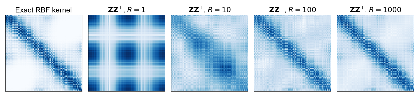
应用——高斯核近似

import matplotlib.pyplot as plt
import numpy as np
from   sklearn.metrics.pairwise import rbf_kernel
from   sklearn.datasets import make_s_curve

fig, axes = plt.subplots(1, 5)
fig.set_size_inches(15, 4)
font = {'fontname': 'arial', 'fontsize': 18}

N    = 1000
D    = 3
X, t = make_s_curve(N, noise=0.1)
X    = X[t.argsort()]
# The RBF kernel is the Gaussian kernel if we let \gamma = 1 / (2 \sigma^2).
K    = rbf_kernel(X, gamma=1/2.)

axes[0].imshow(K, cmap=plt.cm.Blues)
axes[0].set_title('Exact RBF kernel', **font)
axes[0].set_xticks([])
axes[0].set_yticks([])

for R, ax in zip([1, 10, 100, 1000], axes[1:]):
    W    = np.random.normal(loc=0, scale=1, size=(R, D))
    b    = np.random.uniform(0, 2*np.pi, size=R)
    B    = np.repeat(b[:, np.newaxis], N, axis=1)
    norm = 1./ np.sqrt(R)
    Z    = norm * np.sqrt(2) * np.cos(W @ X.T + B)
    ZZ   = Z.T@Z

    ax.imshow(ZZ, cmap=plt.cm.Blues)
    ax.set_title(r'$\mathbf{Z} \mathbf{Z}^{\top}$, $R=%s$' % R, **font)
    ax.set_xticks([])
    ax.set_yticks([])

plt.tight_layout()
plt.show()